Getting Started with natalityr • natalityr

This vignette provides a look at how this package works. Initially, instructions are provided for loading packages, using synthetic or true CDC natality files, and processing data. Then the additional functions for accessing CDC variable documentation and summarizing cesarean rates are explored.

Loading the Package and Processing Datasets

Once the package is installed, simply load in the package with the following line of code.

library(natalityr)

Processing the Synthetic Dataset

The following lines of code pull the synthetic files included within natalityr, and run the package’s processing function.

synthetic_files <- c(
  system.file("extdata","synthetic_2023.txt", 
              package = "natalityr"),
  system.file("extdata",  "synthetic_2024.txt", 
              package = "natalityr"))

processed_synth <- 
  natalityr::prepare_birth_data(
    synthetic_files,
    years_separate = FALSE,
    include_late_term = FALSE)

Downloading and Processing CDC Files

Since the synthetic files are mainly provided as a way to look at natalityr through examples, users will wish to work with the true public use CDC files.

These files can be downloaded from the CDC National Center for Health Statistics website. The package expects the fixed-width .txt files contained within the Birth Data ZIP folders; years 2016 through 2024 are currently supported.

https://www.cdc.gov/nchs/data_access/VitalStatsOnline.htm#Births

Once the files are downloaded, users can pass files into the prepare_birth_data() function. This is demonstrated below using example path names; in practice, users must input their own local file locations.

cdc_files <- c("~/Downloads/Nat2021US.txt", "~/Downloads/Nat2022US.txt",
               "~/Downloads/Nat2023US.txt", "~/Downloads/Nat2024US.txt")

processed_data <- natalityr::prepare_birth_data(cdc_files)

Viewing the Processed Dataset

Once the dataset has been processed, a user will see a dataframe with similar characteristics to the one visualized below.

processed_synth[1:6,
  c("year", "age",
    "race", "delivery",
    "cesarean", "NTSV")]
#> # A tibble: 6 × 6
#>    year   age race  delivery cesarean  NTSV
#>   <int> <dbl> <chr>    <dbl>    <dbl> <dbl>
#> 1  2023    28 2            1        0     1
#> 2  2023    27 3            1        0     1
#> 3  2023    27 4            1        0     1
#> 4  2023    34 1            1        0     1
#> 5  2023    33 2            1        0     1
#> 6  2023    26 3            2        1     1

colnames(processed_synth)
#>  [1] "year"                "time"                "day"                
#>  [4] "hospital"            "age"                 "agecat"             
#>  [7] "nativity"            "race"                "prior_births_living"
#> [10] "prior_births_dead"   "BMI"                 "GWG"                
#> [13] "diabetes_pre"        "diabetes_gest"       "hyper_pre"          
#> [16] "hyper_gest"          "hyper_eclamp"        "previous_cesarean"  
#> [19] "induction"           "augmentation"        "fetalpos"           
#> [22] "labor_attempted"     "delivery"            "payment"            
#> [25] "plural"              "term"                "cesarean"           
#> [28] "labor_all"           "NTSV"

Using the Library to View CDC Codes for Specific Variables

Since the CDC reference documentation can be close to one hundred pages in length, the function can be run below to quickly view the variables specific to this package’s processed dataset.

The following lines look at the raw output for view_birth_codes().

bmi_ref <- view_birth_codes(processed_synth$BMI)
print(bmi_ref, row.names = FALSE)
#>  code                        label
#>     1          Underweight (<18.5)
#>     2    Normal weight (18.5-24.9)
#>     3       Overweight (25.0-29.9)
#>     4        Obesity I (30.0-34.9)
#>     5       Obesity II (35.0-39.9)
#>     6 Extreme obesity III (>=40.0)
#>     9                      Unknown

gwg_ref <- view_birth_codes(processed_synth$GWG)
print(gwg_ref, row.names = FALSE)
#>                                                                                      note
#>  Gestational weight gain (pounds). 98 refers to 98 pounds and over; 99 indicates missing.

Using the Summarizing Cesarean Rate Function

Another function included within this package is summarize_cesarean_rate(), which calculates cesarean delivery rates and Wilson confidence intervals. The user can choose whether to stratify these cesarean rates by one or more variables.

term_rates <- summarize_cesarean_rate(processed_synth, by = c("term"), 
                        NTSV = TRUE,
                        CI_level = 0.95)

print(term_rates)
#> # A tibble: 5 × 7
#>    term total_births missing cesareans cesarean_rate lower_CI upper_CI
#>   <dbl>        <int>   <int>     <int>         <dbl>    <dbl>    <dbl>
#> 1    37            8       0         6         0.75    0.409     0.929
#> 2    38            7       0         6         0.857   0.487     0.974
#> 3    39           10       0         4         0.4     0.168     0.687
#> 4    40            6       0         2         0.333   0.0968    0.700
#> 5    41            9       0         2         0.222   0.0632    0.547

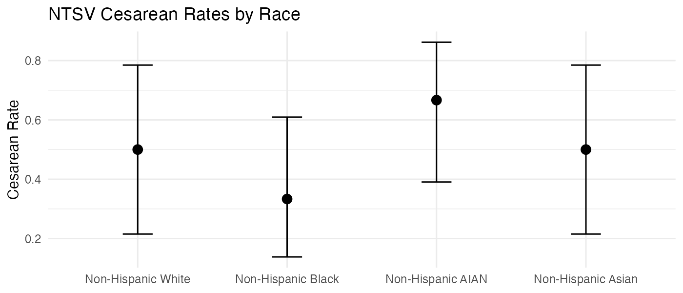
Plotting the Results

Should a user wish to plot the results from summarize_cesarean_rate(), an example on how to do so can be seen below. Also illustrated is how view_birth_codes can be used to create label names in plots for categorical variables.

library(ggplot2)

race_rates <- summarize_cesarean_rate(processed_synth, by = c("race"), 
                        NTSV = TRUE,
                        CI_level = 0.95)

race_codes <- view_birth_codes(processed_synth$race)

race_rates$race <- factor(race_rates$race,
  levels = race_codes$code,
  labels = race_codes$label)

ggplot(race_rates, aes(x = race, y = cesarean_rate)) +
  geom_point(size = 3) +
  geom_errorbar(aes(ymin = lower_CI, ymax = upper_CI),
    width = 0.2) +
  labs(title = "NTSV Cesarean Rates by Race",
    x = NULL,
    y = "Cesarean Rate") +
  theme_minimal()